Attention
Cate has become the ESA Climate Toolbox. This documentation is being discontinued. You can find the documentation on the ESA Climate Toolbox here.
3. Quick Start
This section provides a quick start into Cate by demonstrating how a particular climate use case is performed.
Refer to the User Manual for installing the Cate.
The use case describes a climate scientist wishing to analyse potential correlations between the geophysical quantities Ozone Mole Content and Cloud Coverage in a certain region (see use case description for Relationships between Aerosol and Cloud ECV). It requires the toolbox to do the following:
Access to and ingestion of ESA CCI Ozone and Cloud data (Atmosphere Mole Content of Ozone and Cloud Cover)
Geometric adjustments (coregistration)
Spatial (point, polygon) and temporal subsetting
Visualisation of time series
Correlation analysis, scatter-plot of correlation statistics, saving of image and correlation statistics
3.1. Using the CLI
In the following, a demonstration is given how the use case described above is performed using the Cate’s Command-Line Interface.
3.1.1. Dataset Ingestion
Use ds list to list available products. You can filter them according to some name.
$ cate ds list -n ozone
3 data sources found
   1: esacci.OZONE.day.L3S.TC.GOME-2.Metop-A.MERGED.fv0100.r1
   2: esacci.OZONE.day.L3S.TC.GOME.ERS-2.MERGED.fv0100.r1
   3: esacci.OZONE.mon.L3.NP.multi-sensor.multi-platform.MERGED.fv0002.r1
$ cate ds list -n cloud
14 data sources found
   1: esacci.CLOUD.day.L3U.CLD_PRODUCTS.AVHRR.NOAA-15.AVHRR_NOAA.1-0.r1
   2: esacci.CLOUD.day.L3U.CLD_PRODUCTS.AVHRR.NOAA-16.AVHRR_NOAA.1-0.r1
   3: esacci.CLOUD.day.L3U.CLD_PRODUCTS.AVHRR.NOAA-17.AVHRR_NOAA.1-0.r1
   4: esacci.CLOUD.day.L3U.CLD_PRODUCTS.AVHRR.NOAA-18.AVHRR_NOAA.1-0.r1
   5: esacci.CLOUD.day.L3U.CLD_PRODUCTS.MODIS.Aqua.MODIS_AQUA.1-0.r1
   6: esacci.CLOUD.day.L3U.CLD_PRODUCTS.MODIS.Terra.MODIS_TERRA.1-0.r1
   7: esacci.CLOUD.mon.L3C.CLD_PRODUCTS.AVHRR.NOAA-15.AVHRR_NOAA.1-0.r1
   8: esacci.CLOUD.mon.L3C.CLD_PRODUCTS.AVHRR.NOAA-16.AVHRR_NOAA.1-0.r1
   9: esacci.CLOUD.mon.L3C.CLD_PRODUCTS.AVHRR.NOAA-17.AVHRR_NOAA.1-0.r1
  10: esacci.CLOUD.mon.L3C.CLD_PRODUCTS.AVHRR.NOAA-18.AVHRR_NOAA.1-0.r1
  11: esacci.CLOUD.mon.L3C.CLD_PRODUCTS.MODIS.Aqua.MODIS_AQUA.1-0.r1
  12: esacci.CLOUD.mon.L3C.CLD_PRODUCTS.MODIS.Terra.MODIS_TERRA.1-0.r1
  13: esacci.CLOUD.mon.L3S.CLD_PRODUCTS.AVHRR.multi-platform.AVHRR_MERGED.1-0.r1
  14: esacci.CLOUD.mon.L3S.CLD_PRODUCTS.MODIS.multi-platform.MODIS_MERGED.1-0.r1
Create a new workspace.
$ cate ws new
cate-webapi: started service, listening on localhost:49836
Workspace created.
Open the desired datasets, by providing their name and desired time-span.
$ cate res open cl07 esacci.CLOUD.mon.L3C.CLD_PRODUCTS.multi-sensor.multi-platform.ATSR2-AATSR.2-0.r1
Opening dataset: done
Resource "cl07" set.
$ cate res open oz07 esacci.OZONE.mon.L3.NP.multi-sensor.multi-platform.MERGED.fv0002.r1 2007-01-01 2007-12-30
Opening dataset: done
Resource "oz07" set.
3.1.2. Dataset Variable Selection
To select particular geophysical quantities to work with, use the select_var operation together with
cate res set command:
$ cate res set cfc select_var ds=@cl07 var=cfc
Executing 2 workflow step(s): done
Resource "cfc" set.
$ cate res set oz_tot select_var ds=@oz07 var=O3_du_tot
Executing 2 workflow step(s): done
Resource "oz_tot" set.
Note the at-character “@” in @cl07 and @oz07. This indicates that the input ds of the select_var
operation will be the output of the respective open steps. This establishes a permanent connection
between step open and select_var. In fact, this is the way processing graphs are constructed using
the Cate CLI.
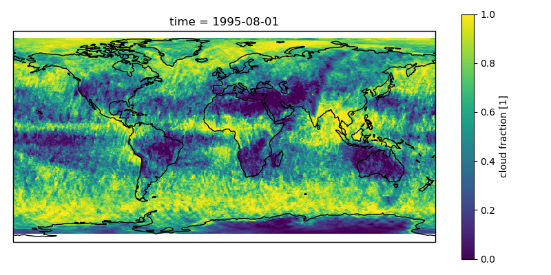
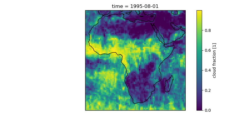
We can plot the datasets and save the plots using the plot_map operation:
$ cate ws run plot_map ds=@cfc var=cfc file=fig1.png
Running operation 'plot_map': Executing 4 workflow step(s)
Operation 'plot_map' executed.
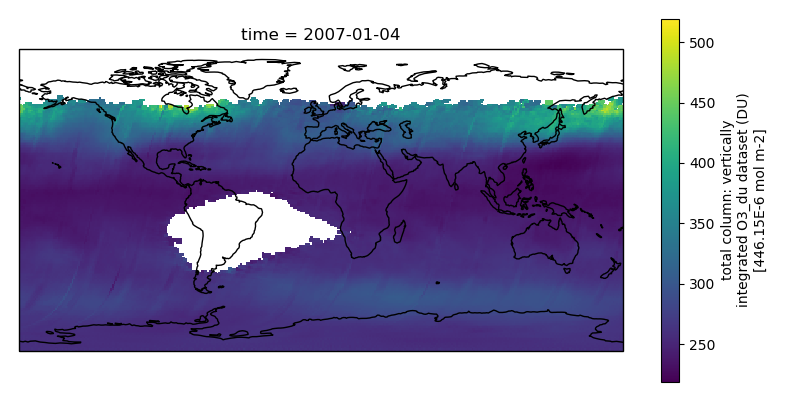
$ cate ws run plot_map ds=@oz_tot var=O3_du_tot file=fig2.png
Running operation 'plot_map': Executing 4 workflow step(s)
Operation 'plot_map' executed.
3.1.3. Co-Register the Datasets
The datasets now have different lat/lon definitions. This can be verified by using cate res print
$ cate res print cfc
<xarray.Dataset>
Dimensions:       (hist_cot: 7, hist_cot_bin: 6, hist_ctp: 8, hist_ctp_bin: 7, hist_phase: 2, lat: 360, lon: 720, time: 12)
Coordinates:
  * lat           (lat) float32 -89.75 -89.25 -88.75 -88.25 -87.75 -87.25 ...
  * lon           (lon) float32 -179.75 -179.25 -178.75 -178.25 -177.75 ...
  * hist_cot      (hist_cot) float32 0.3 1.3 3.6 9.4 23.0 60.0 100.0
  * hist_cot_bin  (hist_cot_bin) float32 1.0 2.0 3.0 4.0 5.0 6.0
  * hist_ctp      (hist_ctp) float32 1100.0 800.0 680.0 560.0 440.0 310.0 ...
  * hist_ctp_bin  (hist_ctp_bin) float32 1.0 2.0 3.0 4.0 5.0 6.0 7.0
  * hist_phase    (hist_phase) int32 0 1
  * time          (time) float64 2.454e+06 2.454e+06 2.454e+06 2.454e+06 ...
Data variables:
    cfc           (time, lat, lon) float64 0.1076 0.3423 0.2857 0.2318 ...
$ cate res print oz_tot
<xarray.Dataset>
Dimensions:       (air_pressure: 17, lat: 180, layers: 16, lon: 360, time: 12)
Coordinates:
  * lon           (lon) float32 -179.5 -178.5 -177.5 -176.5 -175.5 -174.5 ...
  * lat           (lat) float32 -89.5 -88.5 -87.5 -86.5 -85.5 -84.5 -83.5 ...
  * layers        (layers) int32 1 2 3 4 5 6 7 8 9 10 11 12 13 14 15 16
  * air_pressure  (air_pressure) float32 1013.0 446.05 196.35 113.63 65.75 ...
  * time          (time) datetime64[ns] 2007-01-04 2007-02-01 2007-03-01 ...
Data variables:
    O3_du_tot     (time, lat, lon) float32 260.176 264.998 267.394 265.048 ...
$ cate op list --tag geom
2 operations found
   1: coregister
   2: subset_spatial
will list all commands that have a tag that matches ‘*geom*’.
To find out more about a particular operation, use cate op info
$ cate op info coregister

Operation cate.ops.coregistration.coregister
============================================

Perform coregistration of two datasets by resampling the replica dataset unto the
grid of the master. If upsampling has to be performed, this is achieved using
interpolation, if downsampling has to be performed, the pixels of the replica dataset
are aggregated to form a coarser grid.

The returned dataset will contain the lat/lon intersection of provided
master and replica datasets, resampled unto the master grid frequency.

This operation works on datasets whose spatial dimensions are defined on
pixel-registered and equidistant in lat/lon coordinates grids. E.g., data points
define the middle of a pixel and pixels have the same size across the dataset.

This operation will resample all variables in a dataset, as the lat/lon grid is
defined per dataset. It works only if all variables in the dataset have lat
and lon as dimensions.

For an overview of downsampling/upsampling methods used in this operation, please
see https://github.com/CAB-LAB/gridtools

Whether upsampling or downsampling has to be performed is determined automatically
based on the relationship of the grids of the provided datasets.

Version: 1.1

Inputs:
  ds_master (Dataset)
      The dataset whose grid is used for resampling
  ds_replica (Dataset)
      The dataset that will be resampled
  method_us (str)
      Interpolation method to use for upsampling.
      default value: linear
      value set: ['nearest', 'linear']
  method_ds (str)
      Interpolation method to use for downsampling.
      default value: mean
      value set: ['first', 'last', 'mean', 'mode', 'var', 'std']

Output:
  return (Dataset)
      The replica dataset resampled on the grid of the master
      add history: True
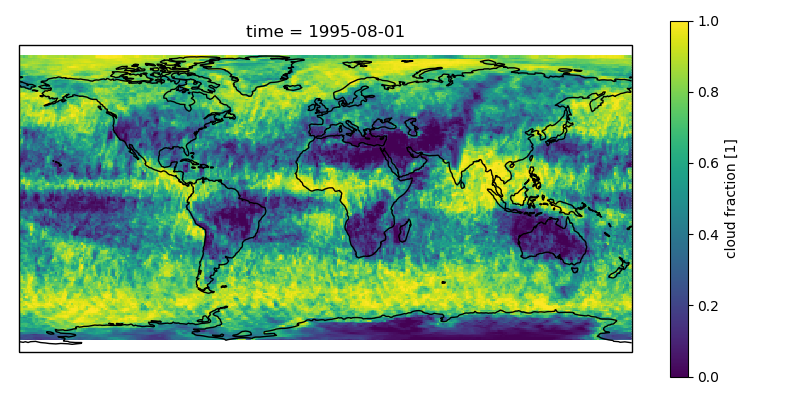
To carry out coregistration, use cate res set again with appropriate operation parameters
$ cate res set cfc_res coregister ds_master=@oz_tot ds_replica=@cfc
Executing 5 workflow step(s): done
Resource "cfc_res" set.
$ cate ws run plot_map ds=@cfc_res var=cfc file=fig3.png
Running operation 'plot_map': Executing 5 workflow step(s)
Operation 'plot_map' executed.
3.1.4. Spatial Filtering
To filter the datasets to contain only a particular region use the subset_spatial operation.
$ cate res set oz_africa subset_spatial ds=@oz_tot region=-20,-40,60,40
Executing 3 workflow step(s): done
Resource "oz_africa" set.
$ cate res set cc_africa subset_spatial ds=@cfc_res region=-20,-40,60,40
Executing 6 workflow step(s): done
Resource "cc_africa" set.
$ cate ws run plot_map ds=@cc_africa var=cfc file=fig4.png
Running operation 'plot_map': Executing 7 workflow step(s)
Operation 'plot_map' executed.
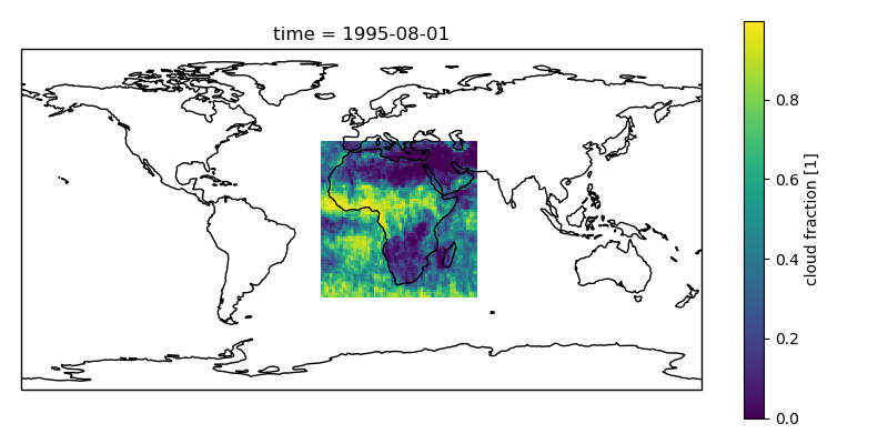
$ cate ws run plot_map ds=@cc_africa var=cfc region=-20,-40,60,40 file=fig5.png
Running operation 'plot_map': Executing 7 workflow step(s)
Operation 'plot_map' executed.
3.1.5. Temporal Filtering
To further filter the datasets to contain only a particular time range, use subset_temporal operation
$ cate res set oz_africa_janoct subset_temporal ds=@oz_africa time_range=2007-01-01,2007-10-30
$ cate res set cc_africa_janoct subset_temporal ds=@cc_africa time_range=2007-01-01,2007-10-30
3.1.6. Extract Time Series
We’ll extract spatial mean timeseries from both datasets using tseries_mean operation.
$ cate res set cc_africa_ts tseries_mean ds=@cc_africa_janoct var=cfc
Executing 8 workflow step(s): done
Resource "cc_africa_ts" set.
$ cate res set oz_africa_ts tseries_mean ds=@oz_africa_janoct var=O3_du_tot
Executing 5 workflow step(s): done
Resource "oz_africa_ts" set.
This creates datasets that contain mean and std variables for both time-series.
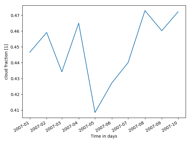
3.1.7. Time Series Plot
To plot the time-series and save the plot operation can be used together with cate ws run operation:
$ cate ws run plot ds=@cc_africa_ts var=cfc file=fig6.png
Running operation 'plot': Executing 11 workflow step(s)
Operation 'plot' executed.
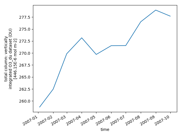
$ cate ws run plot ds=@oz_africa_ts var=O3_du_tot file=fig7.png
Running operation 'plot': Executing 11 workflow step(s)
Operation 'plot' executed.
3.1.8. Product-Moment Correlation
To carry out a product-moment correlation on the mean time-series, the pearson_correlation_scalar operation can be used.
$ cate op list --tag correlation
2 operations found
  0: pearson_correlation
  1: pearson_correlation_scalar
$ cate res set pearson pearson_correlation ds_y=@cc_africa_ts ds_x=@oz_africa_ts var_y=cfc var_x=O3_du_tot
Executing 12 workflow step(s): done
Resource "pearson" set.
This will calculate the correlation coefficient along with the associated p_value for both mean time-series.
We can view the result using cate res print, or save it using cate res write:
$ cate res print pearson
{'corr_coef': -0.2924, 'p_value': 0.4123}
$ cate res write pearson pearson.txt
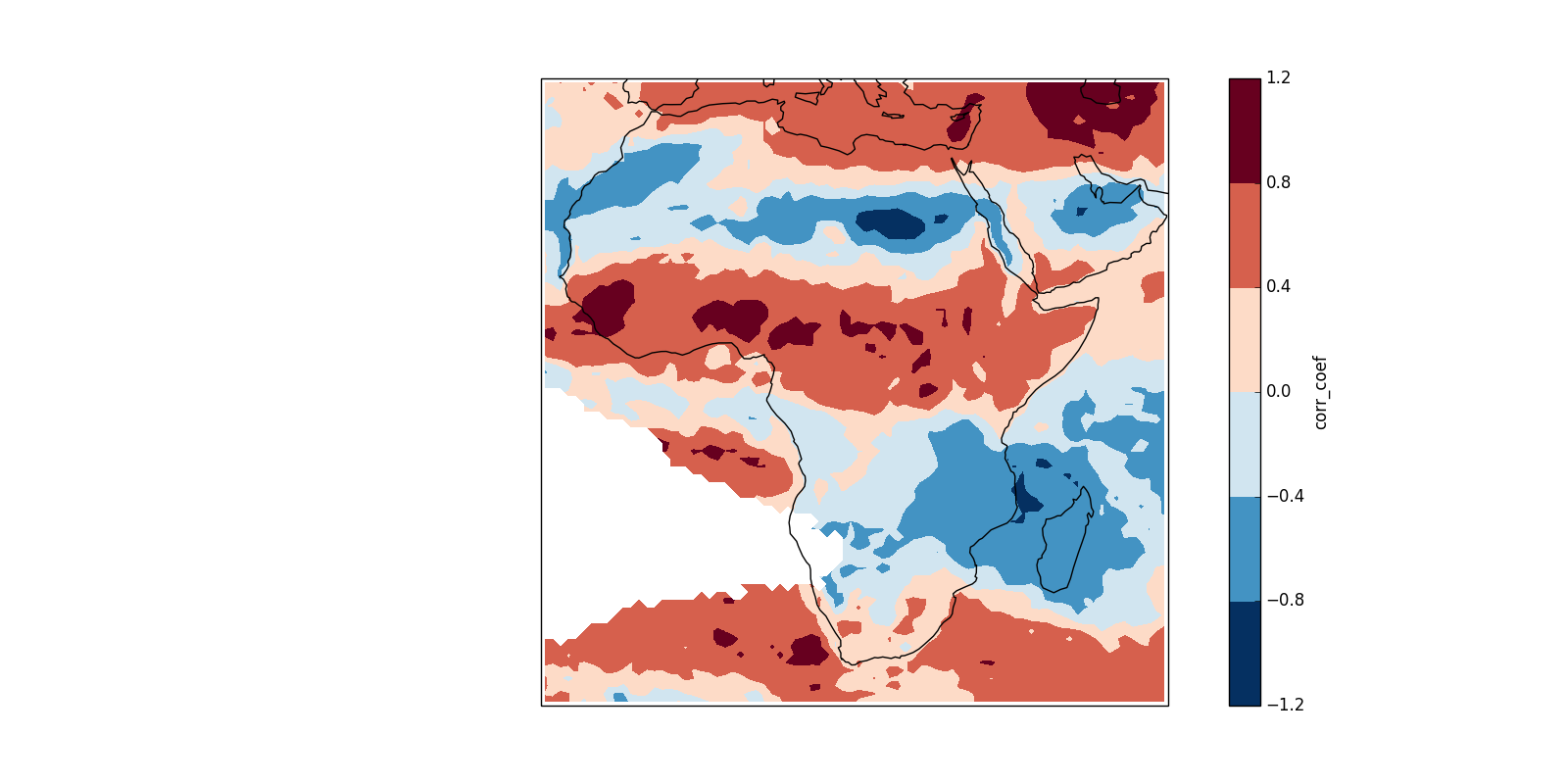
To carry out a pixel by pixel correlation of two coregistered time/lat/lon datasets such
that the result is a map of correlation coefficients or the corresponding
probability values, one can use pearson_correlation:
$ cate res set pearson_map pearson_correlation ds_y=@cc_africa_janoct ds_x=@oz_africa_janoct var_y=cfc var_x=O3_du_tot
Executing 10 workflow step(s): done
Resource "pearson_map" set.
$ cate ws run plot_map ds=@pearson_map var=corr_coef lat_min=-40 lat_max=40 lon_min=-20 lon_max=60 file=fig8.png
Running operation 'plot_map': Executing 13 workflow step(s)
Operation 'plot_map' executed.
3.2. Using the API
A demonstration of how to apply the Cate’s Python API to the use case described here is given in the cate-uc09.ipynb notebook example.