4.4. Cate App
Applies to Cate App web application, version 2.0.0 and higher.
4.4.1. Overview
Cate App is a web application and is intended to serve as a graphical user interface (GUI) for the CCI Toolbox.
It provides to users access to the Cate software without any installation and configuration.
It provides all the Cate CLI and almost all Cate Python API functionality through a interactive and user friendly interface and adds some unique imaging and visual data analysis features.
The basic idea of Cate App is to allow access all remote CCI data sources and calling all Cate operations through a consistent interface. The results of opening a data source or applying an operations is usually an in-memory dataset representation - this is what Cate calls a resource. Usually, a resource refers to a (NetCDF/CF) dataset comprising one or more geo-physical variables, but a resource can virtually be of any (Python) data type.
Attention
The latest version of Cate App SaaS is available at: https://cate.climate.esa.int The Cate SaaS cloud service is free to use. User just need to register. Cate SaaS provides some computational resources free of charge, however service capacities might be throttled depending on the number of concurrent users logged into the system.
The Cate App user interface basically comprises panels, views, and a menu bar:
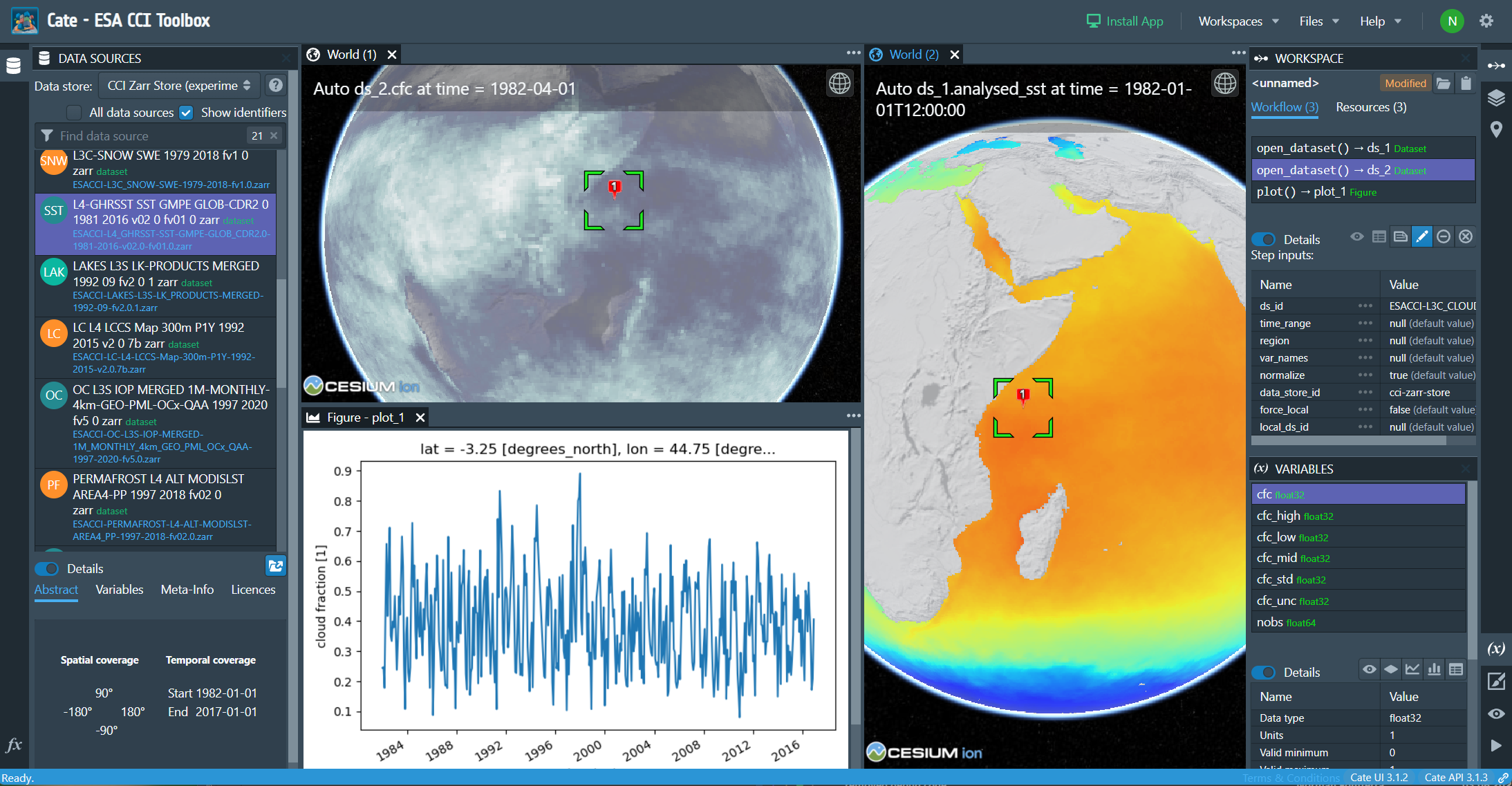
Fig. 4.1 Cate App
4.4.1.1. Panels
When run for the first time, the initial layout and position of the panels, as shown in gui_initial,
reflects what just has been described above with respect to data sources, operations, resources/datasets, and variables:
On the upper left, the DATA SOURCES panel to browse, download and open both local and remote data sources, including data from ESA CCI Open Data Portal;
On the lower left, the OPERATIONS panel to browse and apply available operations;
On the upper right, the WORKSPACE panel to browser and select available resources and workflow steps resulting from opening data sources and applying operations;
On the lower right, the VARIABLES panel to browse and select the geo-physical variables contained in the selected resource.
Other panels are initially hidden. They are
On the upper right, the LAYERS panel, to manage the imagery layers displayed on the active World view;
On the upper right, the PLACEMARKS panel, to manage user-defined placemarks, which may be used as input to various operations, e.g. to create time series plots;
On the lower right, the STYLES panel, to adjust the styles of the selected layer or entity;
On the lower right, the VIEWS panel, to display and edit properties of the currently active view. It also allows for creating new World views;
On the lower right, the TASKS panel, to list and possibly cancel running background tasks.
Each panel’s visibility can be controlled by left- and right-most panel bars. Click on a panel icon to toggle its visibility. Between two panels, there are invisible, horizontal split bars. Move the mouse pointer over the split bar to see it turning into a split cursor, then drag to change the vertical split position. In a similar way, there are invisible, vertical split bars between the tool panels and the views area. Move the mouse cursor over them to find them.
4.4.1.2. Views
The central area is occupied by views that can be arranged in rows and columns. Cate currently offers three view types:
The world view, displaying imagery data originaling from data variables and placemarks on either a 3D globe or a 2D map;
The table view, displaying tabular resource and variable data in a table;
The figure view, displaying plots from special figure resources resulting from the various plotting operations.
There may be multiple views stacked in a row of tabs, where each tab represents a view. One view within a tab row is selected and visible. The selected view can be split horizontally or vertically by dedicated icon buttons on the right of the tab row header. A split view can be stacked again by the drop down menu (…) on the right-most position of the the row tab header.
There is always a single active view indicated by the blueish view header text. To activate a view, click its header text. The active view provides a context for various commands, for example all interactions with the LAYERS and VIEW panels are associated with the active view.
Initially, a single World view is opened and active.
4.4.1.3. Menu Bar
Cate’s menu currently comprises the Workspaces, Logout, and Preferences menus. The Workspaces menu comprises Workspace-related commands:
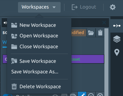
Fig. 4.2 Cate App’s Workspaces menu
Menu item |
Description |
|---|---|
New Workspace |
Creates a new scratch workspace. Scratch workspaces are not-yet-saved workspaces. |
Open Workspace |
Opens an existing workspace. Will open a dialog to select a workspace directory. |
Close Workspace |
Close current workspace and create a new scratch workspace. |
Save Workspace |
Save current workspace it its directory. Will delegate to Save Workspace As if it hasn’t been saved before. |
Save Workspace As |
Opens a dialog to choose a new empty, directory in which the current workspace data will be saved. This will become the current workspace directory. |
Delete Workspace |
Opens a dialog where users can delete existing workspaces. |
More information regarding workspaces can be found in section Workflows, Resources, and Workspaces.
More information regarding Preferences can be found in section Preferences Dialog.
4.4.2. Reference
4.4.2.1. Index
4.4.2.2. DATA SOURCES Panel
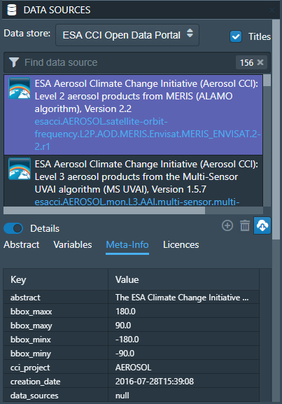
Fig. 4.3 Data Sources panel for ESA CCI Open Data Portal
The DATA SOURCES panel is used to browse, download and open both local and remote data sources published by data stores.
Using the drop-down list located at the top of the panel, it is possible to switch between the the currently available data stores. At the time of writing, two data stores were available in Cate, the remote ESA Open Data Portal, and Local Data Sources representing datasets made available through your file system. Below data stores selector, there is a search field, while typing, the list of data sources published through the selected data store is narrowed down. Selecting a data source entry will allow displaying its Details, namely the available (geo-physical) variables and the meta-data associated with the data source.
In order to start working with remote data from the ESA CCI Open Data Portal data store, there are two options which are explained in the following:
Download the complete remote dataset or a subset and make it a new local data source available from the local data store. Open the dataset from the new local data source. This is currently the recommended way to access remote data as local data stores ensure sufficient I/O performance and are not bound to your internet connection and remote service availability.
Open the remote dataset without creating a local data copy. This option should only be used for small subsets of the data, e.g. time series extractions within small spatial areas, as there is currently no way to observe the data rate and status of data elements already transferred. (Internally, we use the OPeNDAP service of the ESA CCI Open Data Portal.)
After selecting a remote data source, press the Download button to open the Download Dataset* dialog shown in Fig. 4.4 to use the first option.
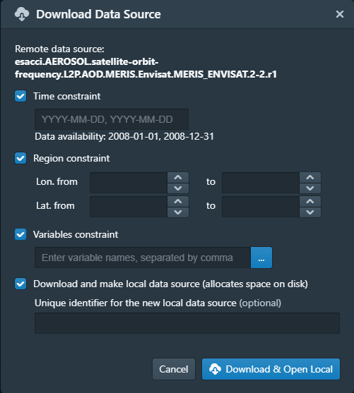
Fig. 4.4 Download Dataset dialog
Here you can specify a number of optional constraints to create a local data source that is a subset of the original
remote one. You can also provide a name for the new data source. By default, the original name will be used, prefixed
by local..
Note
We strongly recommend to set the constraints to limit the overall amount of data to be downloaded
and stored. We are currently not able to pre-compute the amount of data and the time it will take to
fully download it.
Also note, that downloading remote data may require a lot of free space on your local system.
By default, Cate stores this data in the user’s home directory. On Linux and Mac OS, that is
~/.cate/data_stores, on Windows it is
%USER_PROFILE%\.cate\data_stores.
Use the Preferences Dialog to set an alternative location.
After confirming the dialog, a download task will be started, which can be observed in the TASKS panel.
Once the download is finished, a notification will be displayed and a new local data source will be available for the
local data store.
To choose the second option described above, press the Download button to open the Download Dataset dialog, and then uncheck Download and make local data source (allocates space on disk) as shown in Open Remote Dataset dialog.
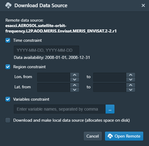
Fig. 4.5 Open Remote Dataset dialog
It provides the same constraint settings as the former download dialog. After confirming the dialog, a task will be started that directly streams the remote data into your computer’s local memory. If the open task finishes, a new dataset resource is available from the WORKSPACE Panel.
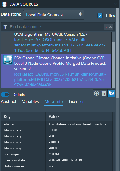
Fig. 4.6 Data Sources panel for local
Switching the data store selector to Local Data Sources lists all currently available local data sources as shown in Fig. 4.6. These are the ones downloaded from remote sources, or ones that you can create from local data files.
Press the Add button to open the Add Local Data Source dialog that is used to create a new local data source.
A data source may be composed of one or more data files that can be stacked together along their time dimension
to form a single unique multi-file dataset. At the time of writing, only NetCDF (*.nc) data sources are supported.
Pressing the Open button will bring up the Open Local Dataset dialog as shown in Fig. 4.7 below:
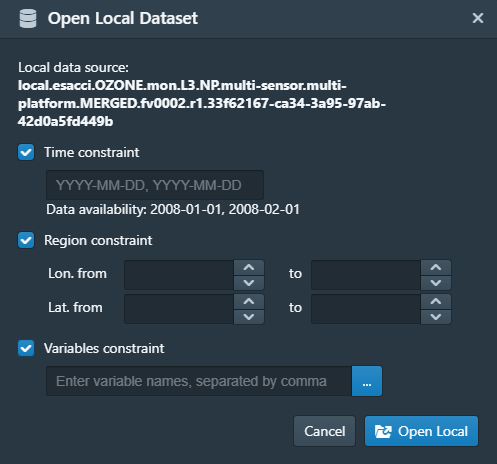
Fig. 4.7 Open Local Dataset dialog
Confirming the dialog will create a new in-memory dataset resource which will be available from the WORKSPACE panel as shown in Fig. 4.12.
Note, that Cate will load into memory only those slices of a dataset, which are required to perform some action. For example, to display an image layer on the 3D Globe view, Cate only loads the 2D image for a given time index, although the dataset might be composed of multiple such 2D images that form a time series and / or a stack of atmospheric layers.
4.4.2.3. OPERATIONS Panel
The OPERATIONS panel is used to browse and apply available operations. The term operations as used in the Cate context includes functions that
read datasets from files;
manipulate these dataset;
plot datasets;
write datasets to files.
The Details section provides a description about the operation including its inputs and outputs.
Note
To programmers: At the time of writing, all Cate operations are plain Python functions.
To let them appear in Cate’s GUI and CLI, they are annotated with additional meta-information.
This also allows for setting specific operation input/output
properties so that specific user interfaces for a given operation is genereted on-the-fly.
You might be interested to take a look at the various functions in the modules of
the cate.ops Python package of Cate.
These functions all use Python 3.5 type annotations and Cate decorators @op, @op_input,
@op_output to add that meta-information to turn it into Cate operations.
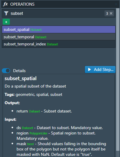
Fig. 4.8 Operations panel
Pressing the Add Step… button will bring up a dialog that let’s you enter the operation’s parameter values. For most parameter types (numeric, boolean, text), an input field is provided. For the ones that don’t have a dedicated input field, a resource selector is provided that let’s you select a resource from a drop-down list. Only resources are listed whose data type match the required parameter type. Most commonly, these will be resources of type
Dataset: N-dimensional, gridded data as originating from NetCDF file sets or OPeNDAP servicesDataFrame: two-dimensional, tabular data from CSV filesGeoDataFrame: similar toDataFramebut include geometry data and are originating from ESRI Shapefiles and GeoJSON services.
Note that every parameter value can be set to a resource by checking the switch to right of the parameter field. This will exchange the input field by a resource selector.
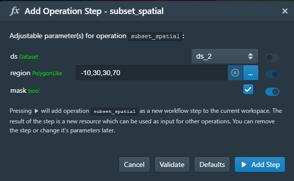
Fig. 4.9 New Operation Step dialog
After pressing the Add Step button, the operation is being invoked and a new workflow step will be added to the workspace. For any operations returning a value a new resource will be added as well.
The new workflow step and the new resource, if any, are shown in the WORKSPACE panel.
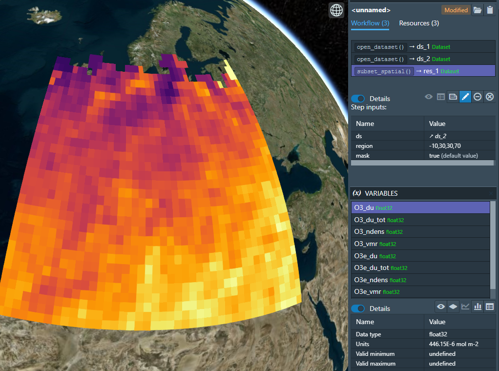
Fig. 4.10 New Operation Step in WORKSPACE Panel
Note
Some operations allow or require entering a path to a file or a directory location. When you pass a relative path, it is meant to be relative to the current workspace directory.
4.4.2.4. WORKSPACE Panel
The WORKSPACE panel is used to manage the current Cate workspace whose name is displayed in the header line of the panel. To the right of the workspace name there is an indicator whether the workspace is modified or not.
In the upper left of the panel are two tools buttons that allow for * opening the workspace directory in your operating system’s file explorer; * copying the workspace workflow into the operating system’s clipboard as Python script, shell script or in JSON format.
The workflow steps and resources of the current workflow are shown in the respective Workflow and Resources sub-panels.
4.4.2.4.1. Workspace / Workflow Panel
This panel lists all the workflow steps originating from opening datasets and applying operations in chronological order. The Details section displays the used parameter values of a selected workflow step.

Fig. 4.11 Workspace / Workflow panel
4.4.2.4.2. Workspace / Resources Panel
This panel lists all the data resources originating from workflow steps. The Details section displays the properties and metadata of the selected data resource.
A data resource may contain any number of data variables. This is usually the case for any resource of type
Dataset or DataFrame. The contained variables of a selected data resource are shown in the VARIABLES panel.
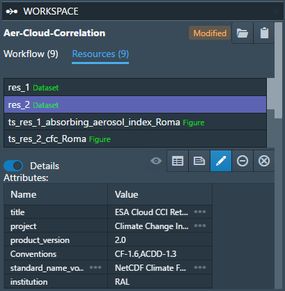
Fig. 4.12 Workspace / Resources panel
The toolbar to the lower right of the list of workflow steps or resources offers the following functions (in order):
Show figure. Shows the associated data resource in a figure view. Only enabled if the resource is of type
Figurewhich is the is for example the case for the variousplot_<type>()operations.Show table: Shows the associated data resource in a table view if it is two-dimensional data.
Edit resource / workflow step properties: Brings up a dialog which lets you rename a resource and make a resource persistent within the workspace. The latter can drastically speed up workspace loading especially for data resources that are expensive to recompute.
Edit operation parameters of a selected workflow step or resource: Brings up a the Edit Operation Step dialog similar to the New Operation Step dialog. Confirming the dialog by pressing Apply will invoke workflow step and compute a new resource value. All workflow step that depend on this resource will also be executed again possibly triggering other workflow step executions.
Remove a selected workflow step or resource. Removal will fail if other steps depend on it.
Clean the current workspace which will remove all steps and resources.
4.4.2.5. VARIABLES Panel
The VARIABLES panel lists the data variables of a selected resource in the WORKSPACE panel. The list entry shows the variable’s name and its data type. When available, the value of each variable of the selected layer will be displayed next to its name after placing the mouse cursor at a point on the globe for ~600ms.
The toolbar to the lower right of the list of variables offers the following functions (in order):
Toggle layer visibility: if the variable can be displayed as an image layer in the 3D globe view.
Add new image layer: adds the selected variable as an image layer to the active world view, if any.
Create time series plot from selected placemark. Adds a new workflow step which calls the
plot()operation.Create histogram plot. Adds a new workflow step which calls the
plot_hist()operation.Show data in table view. Displays 2D variables of type
DataFramein a table view.

Fig. 4.13 Variables panel
4.4.2.6. LAYERS Panel
This panel manages the list of visual layers displayed by the currently active 2D map or 3D world view. Any number of layers can be added to active view. Two are always available:
Selected Variable
Country Borders
The layer Selected Variable displays the data of any selected variable in the VARIABLES panel
if it is gridded and has at least the longitude and latitude dimensions (names lon and lat).
The toolbar to the lower right of the layer list offers the following functions (in order):
Add a new layer (currently you can add layers for other variables available in your workspace)
Remove the selected layer
Move selected layer up to render it on top of others
Move selected layer down so other layers are rendered on top of it
The Details of the LAYERS panel lists several layer settings:
Data selection with this configuration one can quickly browse through the dataset based on the layer index.
Layer split with this setting, user can create a split line with one side of the line showing the globe with the selected layer and the other side showing only the globe.
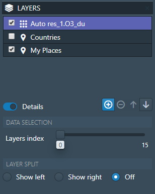
Fig. 4.14 Layers Panel
4.4.2.7. PLACEMARKS Panel
This panel manages a list of placemarks - points, lines, polygons, or boxes that have a name and a geographical coordinate. Placemarks can be used to create time series plots and to extract data at a given point or area. The toolbar to the lower right of the list of placemarks offers the following functions (in order):
Add a new marker
Add a new polyline
Add a new polygon
Add a new box
Remove a selected placemark
Locate the selected placemark on the map
Copy name and/or coordinates of selected placemark to clipboard
In addition to these buttons, there is also a Details toggle button to display or allow modification of the selected placemark. What can be modified depends on which type of placemark is selected.
To add a new marker, click New marker button (the left-most), and then click any point on the Globe. A new entry is added to the list of placemarks in Placemarks Panel. When the Details toggle is enabled, you can modify the name and coordinates (in longitude and latitude) of this marker.

Fig. 4.15 Placemarks Panel - Marker details
To add a new polyline, click New polyline button (the second left-most). Click a point in the Globe to start the line, and then click the next n-lines as you wish. To finish, double-click at your final point. When the Details toggle is enabled, you can modify the name of this polyline.
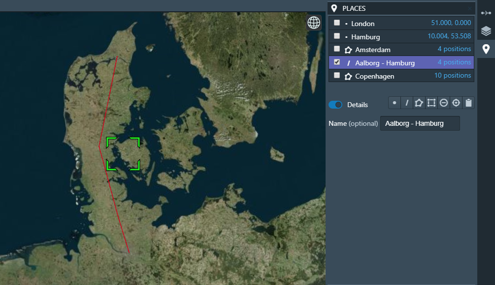
Fig. 4.16 Placemarks Panel - Polyline details
To add a new polygon, click the New polygon button (the third left-most). As when creating a polyline, click a point in the Globe to start the line, and then click the next n-lines as you wish. To finish, double-click at your final point. When the Details toggle is enabled, you can modify the name of this polygon.
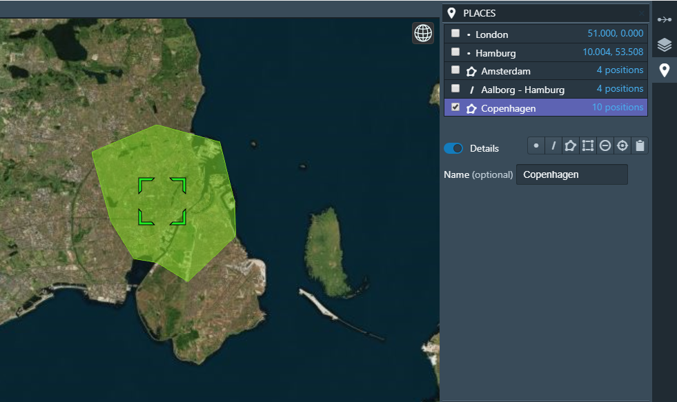
Fig. 4.17 Placemarks Panel - Polygon details
To add a new polygon, click the New box button (the fourth left-most). To start, click a point in the Globe. This will be one of the vertices of the box you are going to create. Drag it to satisfy the region you desire, and click once more to confirm the box selection. When the Details toggle is enabled, you can modify the name of this box.

Fig. 4.18 Placemarks Panel - Box details
To copy the selected placemark to clipboard, click the right-most button. There are three options how the selected placemark can be represented in three different formats: CSV, WKT, and GeoJSON.
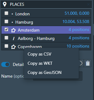
Fig. 4.19 Placemarks Panel - Copy to clipboards
4.4.2.8. STYLES Panel
This panel manages styles that can be applied to the selected layer. It has two different modesdepending on whether an image or a vector layer is selected. Here are the available settings for a vector layer:
Fill controls the fill colour and the opacity of a polygon or a box.
Stroke controls the width, colour, and opacity of the lines surrounding the polygon or the box.
Marker controls the colour, size, and caption of the placemark. The symbol can be either a single digit of number, a letter, or any valid Maki identifier (more information here)
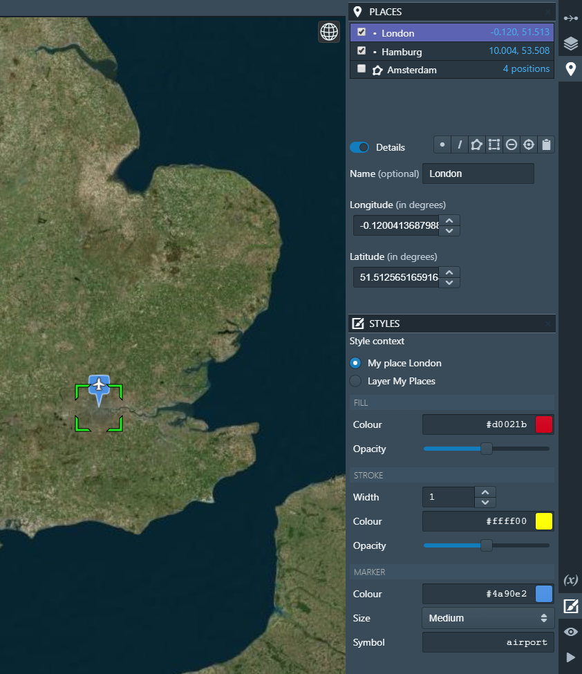
Fig. 4.20 Styles Panel for styling a placemark
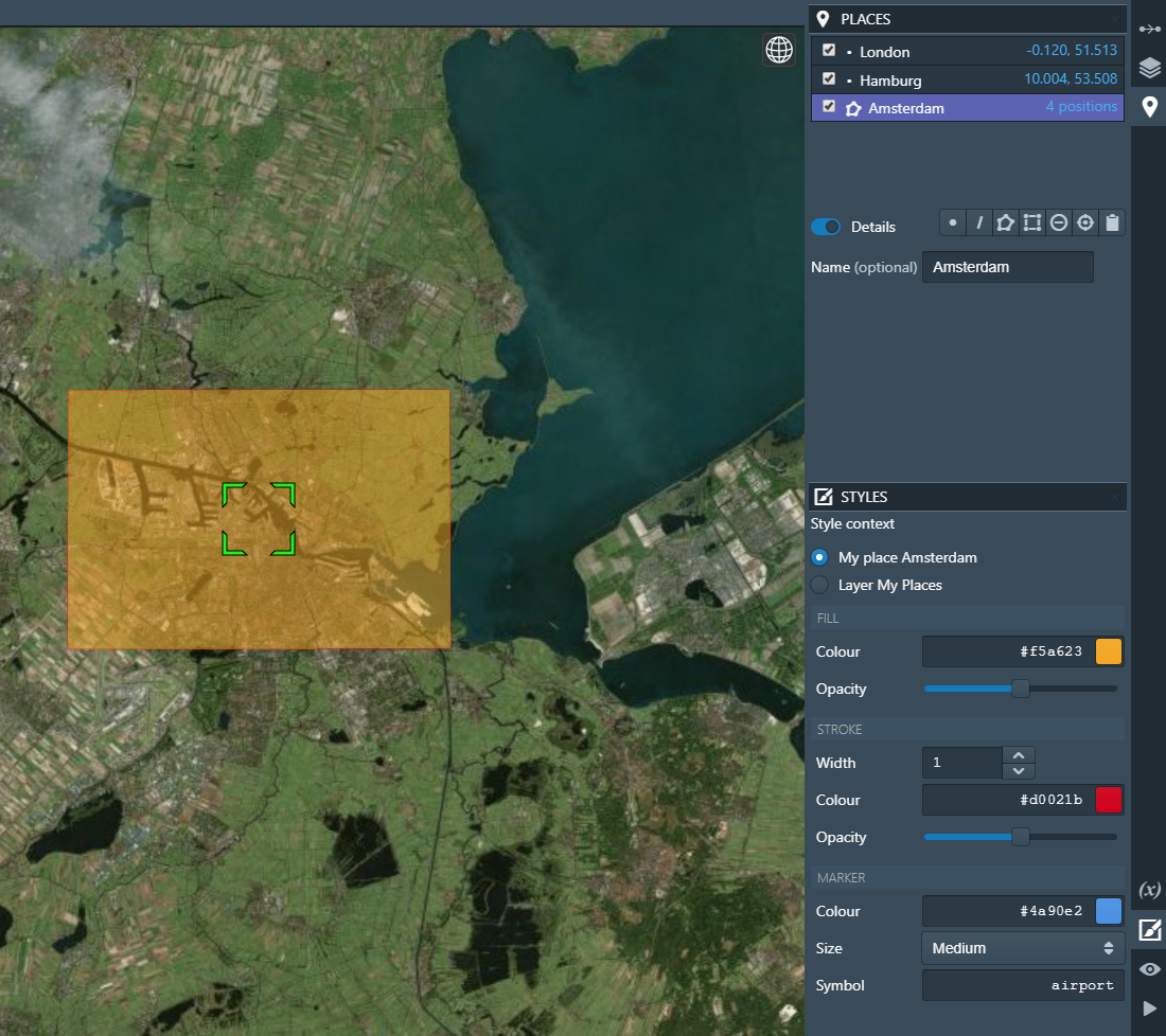
Fig. 4.21 Styles Panel for styling a polygon/box
And here are the available settings for an image layer:
Display Range is the value range to which a given colour map is mapped.
Colour bar is applied to gridded variables.
Alpha Blending is used to mask/fade out the lower half of the display range. With Alpha Blending switched on, the minimum value of the display range corresponds to full transparency while opacity increases until half of the display range is reached.
For any extra dimension of a variable that is not latitude and longitude, an Index into <Dimension> slider is displayed and can be used to selected the dimension’s index to be displayed as layer.
The Opacity controls the opacity of the selected layer
Various Image Enhancement settings, like Brightness, * Contrast*, Hue.
4.4.2.9. VIEW Panel
The VIEW panel shows the settings of the currently active View. The settings depend non the type of the active view.
World Views have the following settings:
Whether to use a 2D map or 3D globe.
The projection for the 2D map.
Whether to show layer titles (currently 3D globe only).
Whether to split the current layer (currently 3D globe only).
Figures Views don’t provide any special settings yet. However, in future releases, you will be able to change plot styles and size.
Table Views also don’t provide any special settings yet. However, in future releases, you will be able to specify the subset of the data ypou want to see in the table.

Fig. 4.22 View Panel
4.4.2.10. TASKS Panel
The TASKS panel shows all active tasks. Long running tasks are usually originating from downloading datasets or performing operations on datasets. Some running tasks may be cancelled, others not.
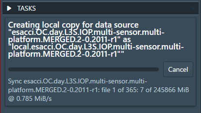
Fig. 4.23 Tasks Panel
4.4.2.11. Preferences Dialog
On the General tab you can specify the following settings:
Whether to reopen the last workspace on startup of Cate
Whether to automatically update the software once a newer version is available
Whether to open a plot view for new Figure resources. If selected and a newly created resource is of type
Figure, a plot view will be opened automatically. Note,Figureresources are created by operations namedplot_<type>().Whether to force offline mode after restart. In this mode Cate does not rely on an internet connection. Therefore the background satellite imagery used for the 2D/3D maps falls back to a static, low resolution map.
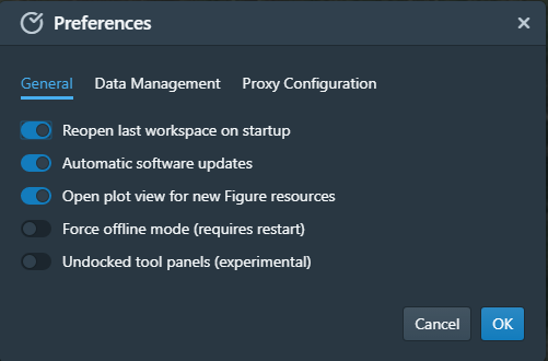
Fig. 4.24 Preferences Dialog / General
On the Data Management tab you can specify the following settings:
The location of the synchronisation directory for remote data store files. This directory is used by Cate for downloading and synchronizing remote data. The location shall ensure sufficient disk space for your type of application and the amount of data required locally.
Whether to use a per-workspace imagery cache which may speed up image display performance. The cache is placed in each workspace directory and requires extra (disk) space.
The resource name prefix which will be used by default for new resources originating from opening datasets or executing operations.
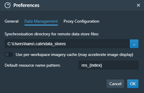
Fig. 4.25 Preferences Dialog / Data Management
On the Proxy Configuration tab you can specify the proxy URL if required.
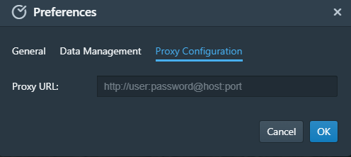
Fig. 4.26 Preferences Dialog / Proxy Configuration
4.4.2.12. Desktop Installation
Cate App may be also be installed as a desktop app by clicking on Install App in the upper right corner:
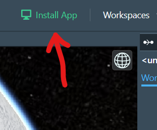
Fig. 4.27 Cate App desktop installation
Once installed, it will open in a new browser window and added to the applications on the desktop, here an example for linux:

Fig. 4.28 Cate App on Desktop
In order to uninstall the Cate App from the machine, launch Cate and it can be removed via Settings:
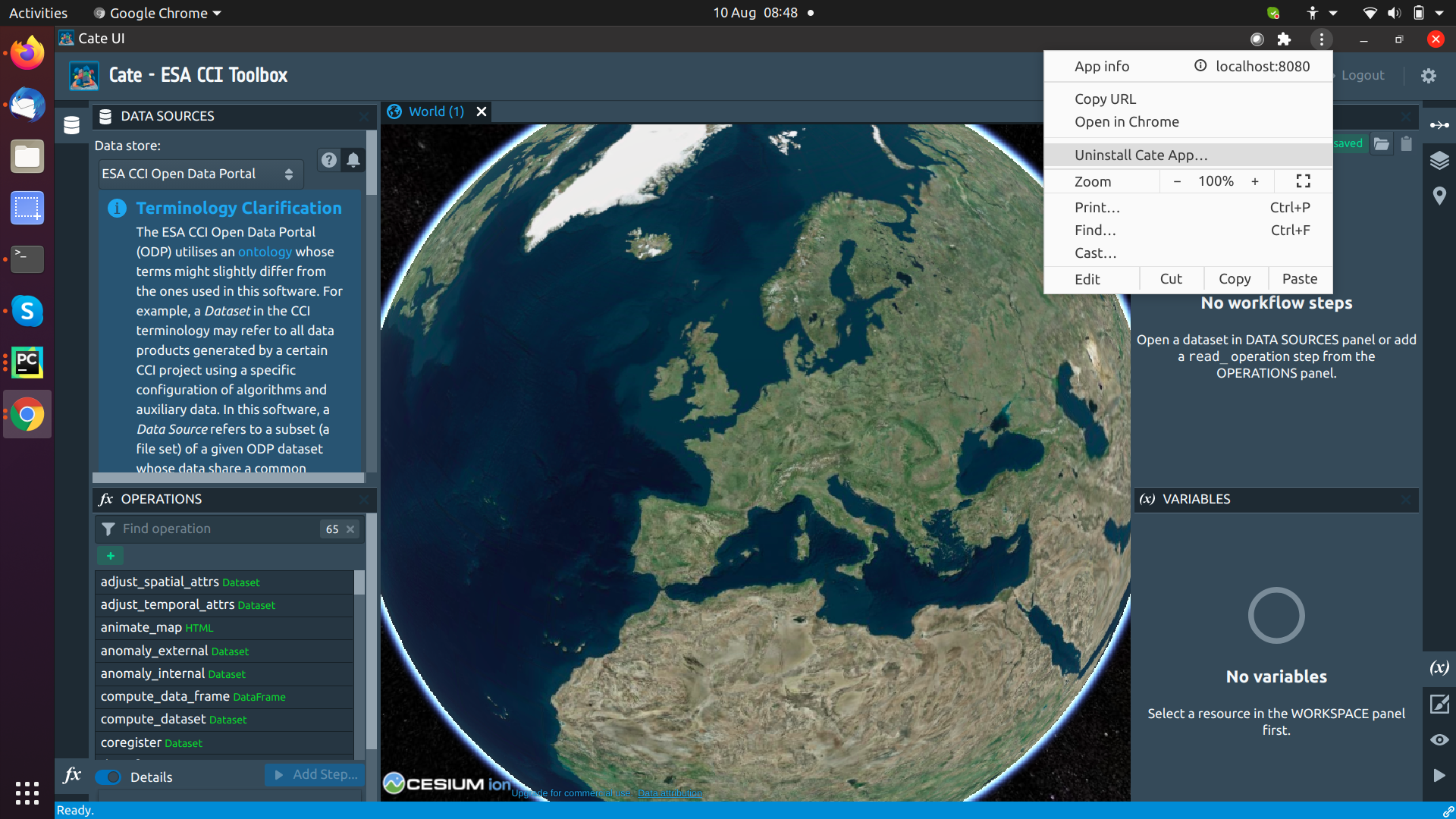
Fig. 4.29 Cate App uninstallation